A Simple Example of Backpropogation in Python

Introduction

Backpropagation is being widely used in neural networks to enable computers learn weights in each layer of a neural network. From mathematics perspective, it is just an implementation of chain rule in Calculus. However, I think its power (in practice) enables the computer to calculate derivative of complex functions (e.g. deep neural networks) without explicitly writing down the mathematical formulas.

In this post, I will use a simple example to illstrate how backprogagtion calculates the derivatives of a function and implement it in python.

Example

The example function used in the post is as follows and our goal is to calculate \(\frac{d}{dx}f\) and \(\frac{d}{dy}f\)

\(f(x,y) = \frac{x+\sigma(y)}{\sigma(x)+(x+y)^{2}}\)
\(\sigma(x) = \frac{1}{1+e^{-x}}\)

A Little Machinery

Before discussing Backpropogation for this function, I have to discuss a property for the sigmoid function \(\sigma(x)\) which will be used later.

\(\frac{d\sigma(x)}{dx} = \sigma(x)(1-\sigma(x))\)

Backpropagation

The spirit of backprogation is

spliting a complex function into several chunks of functions, each of which has a simple derivative with respect to the ’s input.
leverage chain rule to “assemble” each derivative to obtain the final result (\(\frac{d}{dx}f\) and \(\frac{d}{dy}f\) in our example)

In our example, f can be split into the following simple functions (m,n is dummy variables)

sigmoid function \(\sigma(m)\)
\(m+n\)
\(m^{2}\)
\(\frac{1}{m}\)
\(m*n\)

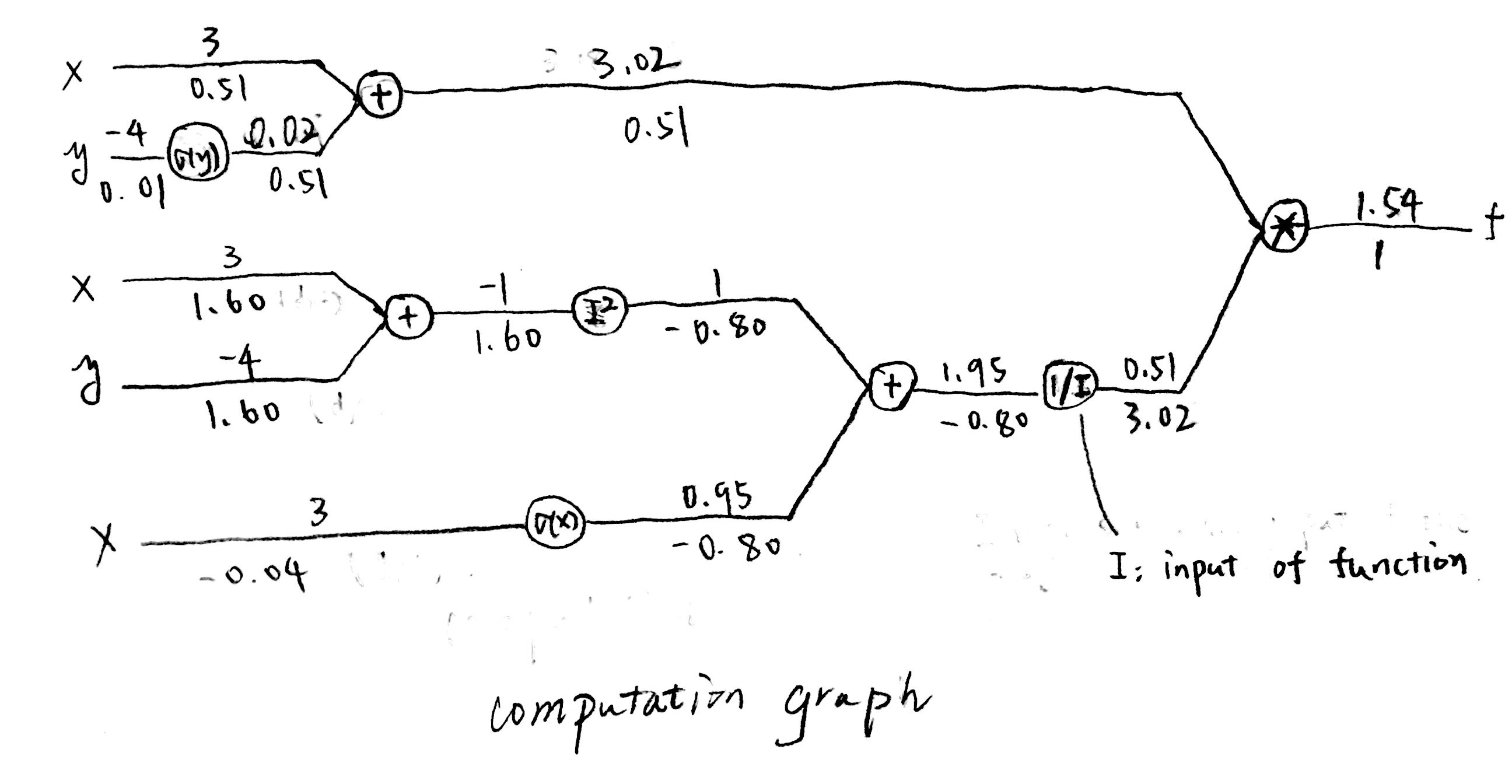
If we assume \(x=3 \ \textrm{and} \ y=-4\), then we can get the following computational graph to obtain the result \(\frac{d}{dx}f\) and \(\frac{d}{dy}f\)

In the computational graph, the input value of an operation (node) is shown on the left to them while the output value is on the right. (above the line, the values under the line are derivative values)
The upstream derivative value of a node is shown on the right to them (below the line). The derivative value with respect to the node is shown on the left to them. It is the product of local derivatives (not shown in graph) and upstream derivative (right).

Python Implementation

Based on the computational graph above, we can therefore implement it in python.

Feedforward Computation

The first computation is feedfoward (from left to right) to compute f(x,y) and each “small” functions.

We save every small functions’ value becasue in the sebsequent backward phase, we need to use it to compute local gradients.

import math
def sig(x):
    """define sigmoid function"""
    return 1.0/(1+math.exp(-x))
x=3
y=-4
sigx = sig(x) # node sigmoid of y
sigy = sig(y) # node sigmoid of x
numer = x+sigy # node numerator (x+sigy)
xandy = x+y # node x+y
xandysqr = xandy*xandy # node (x+y)^2
denom = xandysqr + sigx # node: overall denominator
rec_denom = 1.0/denom # node: reciprcol of denominator
f = numer*rec_denom # function output
print("f output is {0:.2f}".format(f))

## f output is 1.55

Backward Computation (Backpropagation)

In the backward computation phase, we’ll be working from right to left to compute gradients of f(x,y) with respect to each nodes.

The \(\frac{d}{dx}f\) is the sum of all x branches in the computation graph. The same rule applies to y.

df = 1 # derivative of f with respect to f (trivial)
drec_denom = df * numer # derivative with respect to node rec_denom. It is the upstream derivative df * local gradient (multiplication gate)
ddenom = drec_denom * (-1.0/(denom*denom)) # derivative with respect to node denom
dsigx = ddenom * 1 # derivative with respect to sigx
dxandysqr = ddenom * 1 # derivative to node xandsqr
dx1 = dsigx * (sigx*(1-sigx)) # derivative of part of x (one branch of x)
dxandy = dxandysqr * 2*xandy # derivative to node xandy
dx2 = dxandy * 1 # second branch of x
dy1 = dxandy * 1 # first branch of y
dnumer = df * rec_denom # derivative to node numer
dx3 = dnumer * 1 # third branch of x
dsigy = dnumer * 1 # derivative to node sigy
dy2 = dsigy * (sigy*(1-sigy)) # second branch of y
dx = dx1+dx2+dx3 # derivative to variable x
dy = dy1+dy2 # derivative to variable y
print("dx and dy equal to {0:.2f},{1:.2f}".format(dx,dy))

Conclusion

Up to now we have demonstrated how backpropagation can be used and implemented to enable computers to calculate derivatives of a complex function without explicitly writing down the mathematical formula.

The example is based on a note from Standford CS 231n Course. For complete understanding of backpropagation, please go to this link.