Introduction
This is part of my self-note on understanding the derivation of support vector machine (SVM). This short note aims to answer the following question
- What motivats the SVM
- How we formulate the motivation into an mathematical optimization problem
- How to simplify the original optimization problem and solve it by Quadratic Programming (QP)
This short note is based on the understanding of Prof. Hsuan-Tien Lin’s Video on Machine Learning Techniques
Motivation
 Figure is from Prof. Hsuan-Tien Lin’s Slides on ML Techniques
Given the three plots above, there are three classifiers all can separate the positive and negative case. If you can choose one from the three, which one do you want? I guess most of the people will choose the third one. At least I will choose the third one because it is robust to small perturbation of the data. (Think of a scenario that x,y axis represents people’s height and weight. It is highly possible that the data is noisy, say, sometimes you report your height as 184cm or 185cm. In this case a robust(stable) classifier will still make right prediction)
Formulate the Question in Plain English
To achieve such goal above, we have to define what is a good classifier. In SVM, we firstly define margin as the smallest distance between any point and the decision boundary. Then we could say a classifier is better than the other if the its margin is larger than the others’ (Intuitively it means all points can at least perturbate the margin without change in prediction). Another requirement is the usual one that all prediction must be correct. Therefore we can formulate a maximization problem as follows:
s.t. margin defined as minimum distance(sample point i, boundary line/hyperplane)
every sample is correctly classified
Formulate/Translate the Question into Mathematics
In order to solve the optimization problem using mathematics, we have to firstly translate it into mathematics (modeling).
Before that , we have to equip ourselves with some geometry knowledge.
- A hyper plane in \(R^{n}\) can be expressed as (w,b) where \(w^{T}x+b = 0\)
- A line perpendicular to this plane can be expressed as \(w^{T}\)
- The distance between a point \(x_{i}\) in \(r^{n}\) and the hyperplane can be expressed as \(\frac{1}{\|w\|} |w^{T}x_{i}+b|\)
Given sample point is denoted \(x_{i}\) and class is \(y_{i} \in \{-1,+1\}\), the above optimization problem can be translated as
s.t. \(y_{i}(w^{T}x_{i}+b)>0\)
The above problem can be simplified (and equivalent)
s.t. \(y_{i}(w^{T}x_{i}+b)>0\)
because if \(y_{i}(w^{T}x_{i}+b)>0\) holds, then \(y_{i}(w^{T}x_{i}+b)=|y_{i}(w^{T}x_{i}+b)|=|w^{T}x_{i}+b|\) given \(y \in \{-1,1\}\)
Narrow our goal to Simplify the Question
The above maxmium minimum problem is still complicated. By taking a closer look at the problem, we can find if (\(w^{*},b^{*}\)) is a solution, then (\(kw^{*},kb^{*}\)) is also the solution. (i.e. satisfying all constraints and achieves the same optimal value for target function). Therefore, we narrow our goal that we are only interested in the solution making \(min_{i} (w^{T}x_{i}+b)=1\). To illustrate the logic, let’s say we assume (\(w^{*},b^{*}\)) is an optimal solution making \(min_{i} (w^{T}x_{i}+b)=M\). By scaling \(w^{*},b^{*}\) we can always have a new solution \(\frac{w^{*}}{M}, \frac{b^{*}}{M}\) making \(min_{i} (w^{T}x_{i}+b)=1\). Therefore the narrowed version only explores that sort of solution space. And consequently the narrowed version can be much simplified as
s.t. min \(y_{i}(w^{T}x_{i}+b)=1\)
which is equivalent to
s.t. min \(y_{i}(w^{T}x_{i}+b)=1\)
after the following treatment (all of them preserve the equivalence)
- maximization becomes minimization reciprocal,
- adding \(\frac{1}{2}\)
- minimize \(\|w\|\) is equivalent to minimize \(\|w\|^{2}=w^{t}w\)
Relaxation
Unfortunately, the current optimization problem is still hard to solve (due to minimization in constraints). We therefore have to relax the constraint (remove minimization) to \(y_{i}(w^{T}x_{i}+b_{i})>=1\). To illustrate the equivalence of this relaxation. Assume under the new relaxed constraint, we achieve a solution \(w^{'},b^{'}\) and all \(y_{i}(w^{T}x_{i}+b_{i})>1\). By scaling invariance (illustrated above), we can easily get a new \((\frac{w^{'}}{k},\frac{b^{'}}{k})\) making a smaller \(\frac{1}{2}{\|w\|}\). Therefore \(w^{'},b^{'}\) when all \(y_{i}(w^{T}x_{i}+b_{i})>1\) cannot be an optimal solution. There has to be a \(y_{i}(w^{T}x_{i}+b_{i})=1\). Hence the relaxation is equivalent to the original problem.
Solving the Probelm by Quadratic Programming
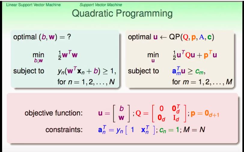
Now current optimization problem after relaxation is stated as follows:
s.t. \(y_{i}(w^{T}x_{i}+b)>=1\)
The above is a Quadratic Programming problem which can be easily solved with a QP solver.

Figure is from Prof. Hsuan-Tien Lin’s Slides on ML Techniques